Macro Regime Model for Multi-Asset Allocation

TL;DR

• •Estimated a 4-state Hidden Markov / regime-switching model on US industrial production and CPI to infer latent business-cycle regimes (Crisis, Stagnation, Expansion, Boom) from 1971 onwards.
• •Used smoothed regime probabilities to study the structure of the cycle (average growth, inflation and asset behaviour in each state), and filtered probabilities for "real-time" trading signals to avoid look-ahead bias.
• •Mapped regimes into an intuitive macro playbook: long duration and gold in Crisis, tilt to credit and quality equities in Stagnation, hold a balanced equity-bond mix in Expansion, and rotate into cyclicals and commodities in Boom.
• •Aligned monthly macro regimes with ETF returns for SPY, TLT, HYG, DBC and GLD, then computed regime-conditional Sharpe ratios and pairwise correlations to see how diversification changes across the cycle.
• •Ran a one-month-lagged, real-time backtest from 2007–2025 and beat an equal-weight benchmark: total return 349% vs 220%, Sharpe 0.88 vs 0.74, and shallower max drawdown (-15.9% vs -24.4%).

What this project demonstrates

• •Building and interpreting regime-switching models. Estimated a Markov-switching growth model in Python (statsmodels) with regime-specific means and variances, selected the number of states via BIC, and distinguished between smoothed and filtered probabilities for analysis vs trading.
• •Translating macro regimes into actual portfolio rules. Turned abstract "Crisis / Boom / Stagnation / Expansion" labels into concrete allocations across equities, duration, credit and commodities, based on regime-level Sharpe and correlation patterns.
• •Handling real-world backtesting issues. Carefully aligned macro and market data at a monthly frequency, lagged signals to avoid look-ahead, and separated the long macro history used to learn regimes from the shorter ETF history used for portfolio testing.
• •Explaining where alpha comes from. Per-regime attribution tables show that most of the excess return is generated by tilting towards defensive assets in Crises and Stagnation and towards commodities and cyclicals in Booms, while correlation analysis documents how stock–bond and stock–commodity relationships flip sign across regimes.
• •Communicating research like a quant PM. Produced a full research pipeline—from FRED/Yahoo data ingestion, feature engineering and HMM estimation through to portfolio construction, backtesting and risk diagnostics—and packaged it in a way that a PM can challenge, modify, or plug into a broader asset-allocation process.

Pipeline

Key Visuals

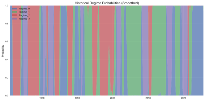
Figure 1: Historical Regime Probabilities (Smoothed). Extended periods of Expansion and shorter but intense episodes of Crisis and Boom appear clearly. Historical episodes like the 1970s, early 1980s double-dip recession, the 2008 global financial crisis, the 2020 Covid shock, and the 2021–2022 inflation episode correspond to intuitive shifts in the regime probabilities.

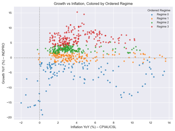
Figure 2: Growth vs Inflation scatter plot colored by ordered regime. The points cluster into distinct clouds. One in the bottom area (negative growth), another around zero growth, and two higher-growth clusters, each with different inflation levels. This visually confirms that the HMM has discovered meaningful macro clusters in the Growth–Inflation plane, rather than arbitrary states.

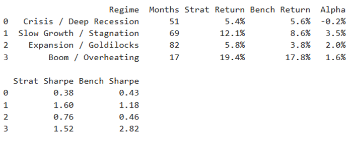
Figure 3: Performance decomposition by macro regime. For each regime, the months classified into that state (using the real-time filtered signal) are isolated, and annualised returns and Sharpe ratios are computed for both the Regime Strategy and the Equal-Weight Benchmark.

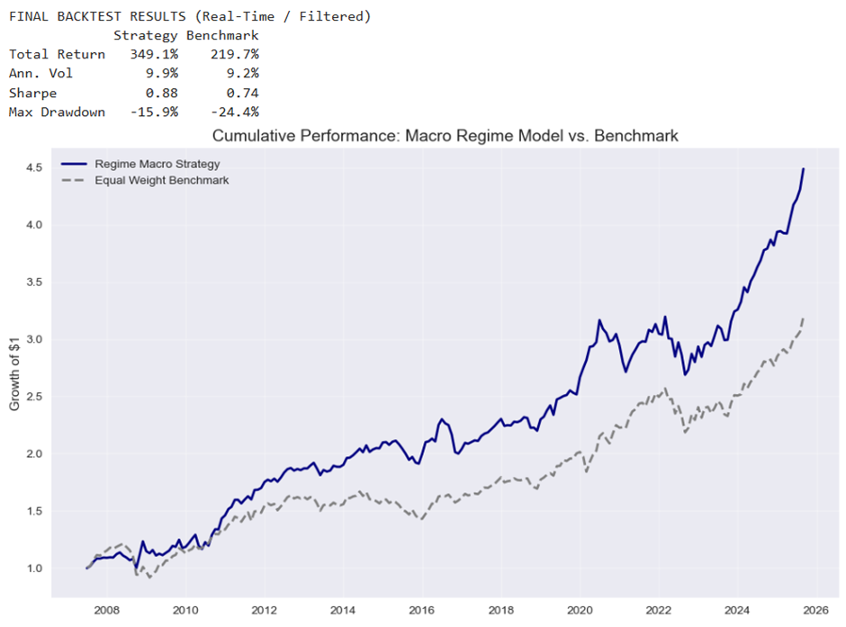
Figure 4: Cumulative performance of the Macro Regime Model vs Benchmark. Over the 2007–2025 test window, the regime strategy grows $1 into roughly $4.5, versus about $3.2 for the benchmark, corresponding to a total return of 349% vs 220%. This outperformance comes with only a slightly higher annualised volatility (9.9% vs 9.2%), so the Sharpe ratio improves from 0.74 to 0.88. The maximum drawdown is also smaller (–15.9% vs –24.4%), meaning the macro-aware allocation not only compounds faster but also experiences shallower peak-to-trough losses.

Appendix: What is a Hidden Markov Model?

The Core Idea

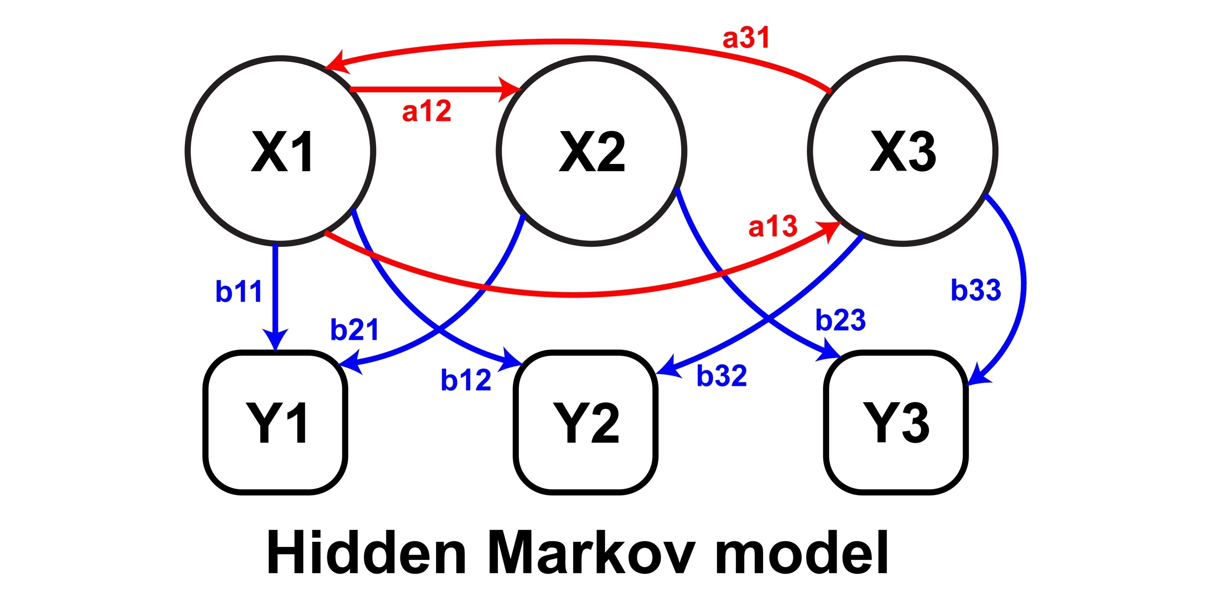
A Hidden Markov Model (HMM) is a statistical model for systems that move between a small number of hidden states over time, while we only observe noisy signals generated by those states.

The "Markov" part means the future state depends only on the current state (not the full history), and the "hidden" part means we never observe the state directly.

How It Works

For each state, the model specifies:

• 1.Emission distribution: A probability distribution for the observed data (for example, a normal distribution with a state-specific mean and volatility).
• 2.Transition matrix: The probability of moving from one state to another at each step.

Inference: What the Model Learns

Given a time series of observations, an HMM uses algorithms like forward–backward to infer two things:

• •The probability of being in each state at every point in time
• •The most likely sequence of states that generated the data

Applications

HMMs are useful whenever you believe there are unobserved regimes driving what you see:

• •Speech recognition: Hidden phonemes generate observed audio signals
• •Fault detection: Hidden machine states generate sensor readings
• •Financial markets: Hidden "economic regimes" (Crisis, Expansion, Boom, Stagnation) influence observable returns and volatility

In this project, we use an HMM to infer 4 latent macro regimes from US growth (industrial production) and inflation (CPI) data, then use these regime probabilities to drive asset allocation decisions across equities, bonds, credit, and commodities.