Macro Factor Model for Sector Rotation & SPY Timing
End-to-end macro factor model using rolling OLS, sector rotation, and SPY timing to test whether macro data can systematically improve equity allocation.
TL;DR
- •Built a rolling OLS macro factor model using 12 US macro indicators (growth, inflation, yield curve, credit, liquidity, USD).
- •Tested both SPY timing (risk-on vs cash) and sector long/short rotation with trend and volatility overlays.
- •Found that the model behaves like a defensive, value-tilted allocator: weak at shorting AI bubbles, but good at capital protection and sector rotation.
- •Produced a full research pipeline: data ingestion → factor engineering → rolling regressions → portfolio construction → performance evaluation.
What this project demonstrates
- •Design and implement an end-to-end systematic macro factor model in Python (pandas, NumPy, Matplotlib).
- •Use relative sector returns instead of absolute returns to reduce market-direction noise.
- •Combine macro factors with price-based trend filters and inverse-volatility weighting to stabilise performance.
- •Critically evaluate regime-dependent models (macro vs AI momentum) and iterate on model design.
Pipeline
Key Visuals

Figure 1: Macro regime dashboard. Standardised growth and inflation (top panel) and financial conditions (bottom panel) over the sample period.
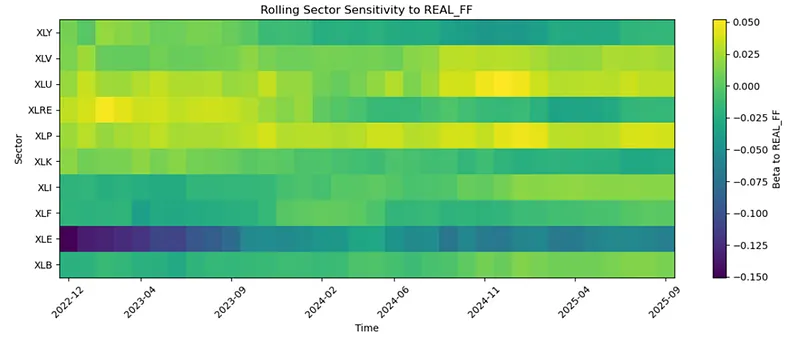
Figure 2: Rolling sector betas to the real policy rate. Heatmap showing the time-varying sensitivity of US sectors to the chosen macro factor (here, the real Fed Funds rate). Warmer colours indicate higher positive sensitivity, colder colours indicate more negative sensitivity, illustrating that sector–macro relationships are not static over time.
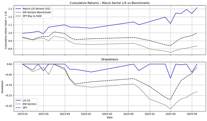
Figure 3: Macro sector long/short strategy versus benchmarks. Top panel shows cumulative returns for the macro sector long/short strategy (V2), an equal-weight sector benchmark, and buy-and-hold SPY. Bottom panel shows corresponding drawdowns. The long/short strategy delivers stronger compounding with shallower drawdowns over the out-of-sample period.
Appendix: Math Foundations
1. Returns and Excess Returns
Let Pi,t be the month-end price of asset i at month t. The simple monthly return is:
Let FFt denote the Effective Fed Funds rate at month t, expressed in annual percent. The monthly risk-free rate is approximated as:
Excess returns (used throughout the model) are:
2. Macro Factor Construction
Let xt denote a generic monthly macro series (e.g. industrial production, CPI).
Year-on-year (YoY) growth:
Acceleration of growth/inflation (6-month change in YoY):
Unemployment gap (labour market slack):
where UNRATĒt is the 5-year rolling mean.
Real policy rate:
Positive values indicate a restrictive real policy stance, negative values an accommodative stance.
3. Lag Structure and Regression Targets
To avoid look-ahead bias, the model uses macro data from month t-1 to forecast returns in month t. The lagged factor vector:
Prediction targets include SPY excess return and sector relative excess returns:
4. Rolling OLS Model
Within each rolling 84-month window, the macro factors are standardised to have zero mean and unit variance. For a given window ending at month t-1:
For each asset i, a linear model is estimated:
The OLS estimate:
5. SPY Timing Rule
The SPY timing strategy uses only the forecast for SPY's excess return. Define a binary exposure signal:
The realised portfolio excess return is:
6. Sector Long/Short Portfolio
Ranking by Predicted Relative Performance:
- Rank sectors by ŷj,t from highest to lowest
- Define the long set Lt as the top N sectors (e.g. N=3)
- Define the short-candidate set St as the bottom N sectors
Trend Filter:
A sector is eligible for shorting only if:
Inverse-Volatility Weights:
Long/Short Return:
7. Performance Statistics
Given a monthly return series {rt} (already expressed in excess-return terms):
Cumulative wealth:
CAGR:
Annualised volatility:
Sharpe ratio:
Maximum drawdown: