Global Multi-Asset Risk Dashboard
Built with Python • pandas • numpy • scikit-learn • Streamlit • Plotly
TL;DR
- •Built a Python-based risk engine that ingests market data and fits rolling regression models to decompose portfolio returns into systematic factor exposures.
- •Designed a "Trader's View" dashboard using Streamlit and Plotly to visualize real-time factor betas and stress test scenarios.
- •Implemented robust statistical methods including Ridge Regression (to handle multicollinearity) and Timezone Synchronization (lagging US factors for Asian markets).
- •Separated concerns with a clean architecture: Data Ingestion → Math Engine → Visualization Layer.
What this project demonstrates
- •End-to-End System Design: Architecting a production-lite application that separates the calculation core (risk_engine.py) from the user interface (main.py).
- •Advanced Data Wrangling: Handling complex time-series issues, specifically aligning US-trading macro factors (like VIX) with Asian-trading assets (like Samsung or Toyota) to prevent look-ahead bias.
- •Statistical Modeling: Using Ridge Regression (L2 Regularization) to stabilize beta estimates in highly correlated market regimes.
- •Scenario Analysis: Moving beyond simple linear shocks by implementing "Coherent Stress Testing"—using historical data to model how factors actually move together during stress events.
Pipeline
The system follows a strict "Data → Engine → View" data flow to ensure modularity and scalability.
Key Visuals
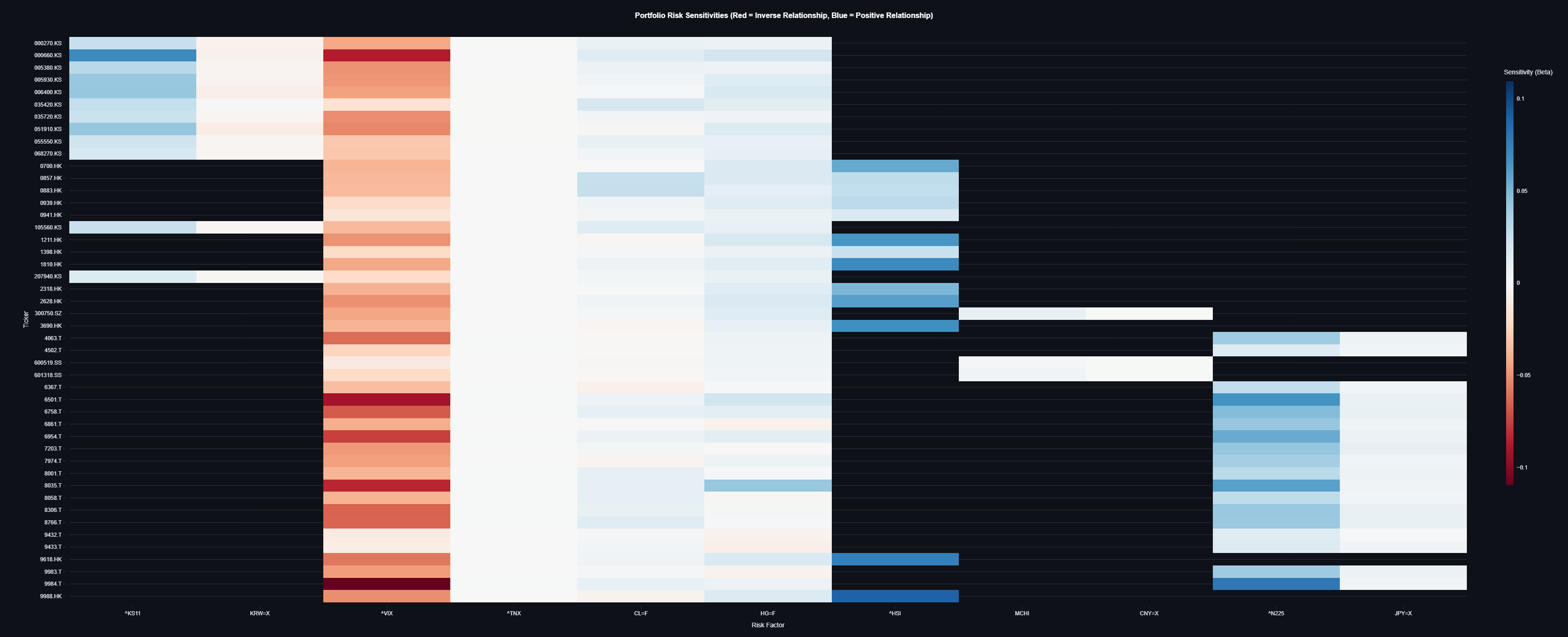
Figure 1: Portfolio risk sensitivities across market factors showing asset-specific exposures.
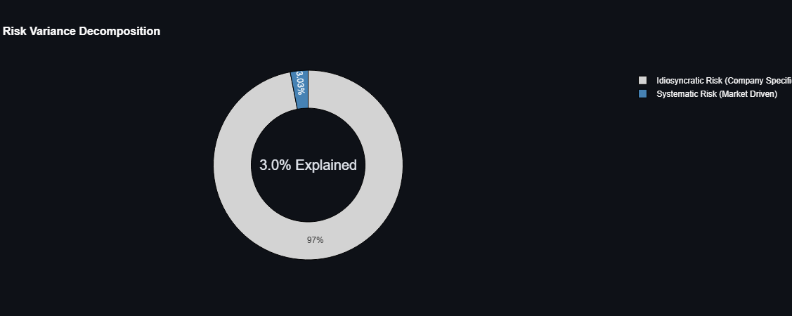
Figure 2: Variance decomposition showing 97% idiosyncratic vs 3% systematic risk.
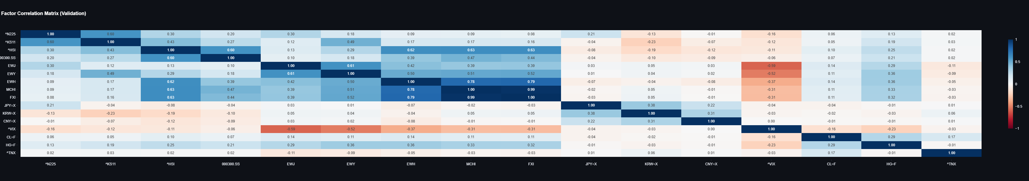
Figure 3: Correlation structure between APAC risk factors revealing diversification opportunities.
Appendix: Math Foundations
1. Factor Risk Decomposition (Ridge Regression)
To understand where risk comes from, we decompose portfolio returns (Rp) into exposures to common risk factors (F). Standard OLS regression often fails in finance due to Multicollinearity (e.g., Interest Rates and Equities moving together).
We use Ridge Regression (L2 Regularization), which adds a penalty term λ to minimize overfitting and stabilize the "jumpiness" of betas:
Result: Stable risk attributions that separate true signal from market noise.
2. Timezone Synchronization
A naive model compares "Today's Nikkei Close" (happens at 3 PM Tokyo) with "Today's S&P 500 Close" (happens 14 hours later). This creates Look-Ahead Bias.
Our engine strictly enforces lag logic based on the asset's region:
3. Coherent Scenario Generation
Instead of guessing how factors move, we use history. To simulate a "20% VIX Spike":
- 1. Identify historical days where VIX was in the top 98th percentile.
- 2. Calculate the average move of all other factors (Rates, Oil, USD) on those specific days.
- 3. Scale those moves proportionally to match the target shock size.